STELLOPT Optimizer Comparision
On this page we provide a simple tutorial exercise to demonstrate how each optimizers works. The basis of this tutorial is a circular cross section tokamak fixed boundary VMEC equilibria with a major radius of 3 and a minor radius of 1 [m]. The optimization goal to to change the major radius to 10 m. While this is a trivial example problem, it highlight the ability of the optimizers to perform a basic task.
The baseline equilibrium
Below you can find the input name list for our VMEC fixed boundary equilibrium
&INDATA
!----- Runtime Parameters -----
  DELT = 1.00000000000000E+00
  NITER = 20000
  NSTEP = 200
  NS_ARRAY = 16 32 64 128
  NITER_ARRAY = 1000 2000 4000 10000
  FTOL_ARRAY = 1.0E-30 1.0E-30  1.0E-30 1.0E-14 !
!----- Grid Parameters -----
  LASYM = F
  NFP = 1
  MPOL = 10
  NTOR = 0
  PHIEDGE = 7.85
!----- Free Boundary Parameters -----
  LFREEB = F
!----- Pressure Parameters -----
  GAMMA = 0.00000000000000E+00
  BLOAT = 0.00000000000000E+00
  SPRES_PED = 0.00000000000000E+00
  PRES_SCALE = 0.00000000000000E+00
  PMASS_TYPE = 'power_series'
  AM = 1.0 -1.0 0.0 0.0 -1.0 1.0
!----- Current/Iota Parameters -----
  NCURR = 0
  PIOTA_TYPE = 'power_series'
  AI = 1.0 0.0 -0.7
!-----  Axis Parameters -----
  RAXIS = 3.00000000000000E+00
  ZAXIS =0.00000000000000E+00
!----- Boundary Parameters -----
  RBC( 0, 0) = 3.0000000000e+00 ZBS( 0, 0) = 0.0000000000e+00
  RBC( 0, 1) = 1.0000000000e+00 ZBS( 0, 1) = 1.0000000000e+00
/
Levenberg-Mardquart Algorithm
In this section we will evaluate the Levenberg-Mardquart algorithm in STELLOPT. We will use the following OPTIMUM name list for STELLOPT
&OPTIMUM
!------------------------------------------------------------------
! OPTIMIZER RUN CONTROL PARAMETERS
!------------------------------------------------------------------
  NFUNC_MAX = 1000
  EQUIL_TYPE = 'VMEC2000'
  OPT_TYPE = 'LMDIF'
  FTOL = 1.0E-4
  XTOL = 1.0E-2
  GTOL = 1.0E-30
  FACTOR = 100.0
  EPSFCN = 1.0E-6
  NOPTIMIZERS = 8
  LKEEP_MINS = T
!------------------------------------------------------------------
! OPTIMIZED QUANTITIES
!------------------------------------------------------------------
  LBOUND_OPT(0,0) = T
  RBC_MIN(0,0)=2.0
  RBC_MAX(0,0)=20.0
  RHO_EXP = 4
!------------------------------------------------------------------
! PLASMA PROPERTIES
!------------------------------------------------------------------
  TARGET_R0 = 10.0 SIGMA_R0 = 1.0
/
We note that while we have specified RBC_MIN and RBC_MAX, these parameters are ignored by the choice of OPT_TYPE as LMDIF. The choice of NFUNC_MAX, FTOL, XTOL, and GTOL only determine when the code ceases to iterate. The choice of EPSFCN will result in a 0.1% perturbation to all quantities in order to calculate the finite difference Jacobian. In the following we show a scan of the FACTOR parameter which sets an initial scaling on how far to move in the descent direction.
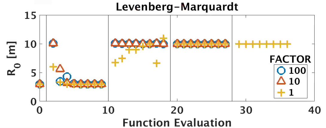
Each simulation was run with an optimizer population of 8. Thus at each stage of the optimization 8 values for R0 were scanned. Vertical lines denote the different iterations of the LMDIF algorithm. We can see that for a factor of 100 or 10, the code appears to achieve R0=10 in the first iteration of the Levenberg algorithm. These cases also achieve their convergence tolerance in the third pass through the optimization loop. For a choice of FACTOR = 1 the code appears to only achieve R0=10 in the second iteration and takes another whole iteration to achieve the desired tolerance.
The Genetic Algorithm with Differential Evolution
In this section we evaluate the Genetic Algorithm with differential evolution in STELLOPT. We will use the following OPTIMUM name list for STELLOPT:
&OPTIMUM
!------------------------------------------------------------------
! OPTIMIZER RUN CONTROL PARAMETERS
!------------------------------------------------------------------
  NFUNC_MAX = 25
  EQUIL_TYPE = 'VMEC2000'
  OPT_TYPE = 'GADE'
  FACTOR = 0.5
  EPSFCN = 0.3
  MODE   = 3
  CR_STRATEGY = 0
  NPOPULATION = 16
  NOPTIMIZERS = 8
  LKEEP_MINS = T
!------------------------------------------------------------------
! OPTIMIZED QUANTITIES
!------------------------------------------------------------------
  LBOUND_OPT(0,0) = T
  RBC_MIN(0,0)=2.0
  RBC_MAX(0,0)=20.0
  RHO_EXP = 4
!------------------------------------------------------------------
! PLASMA PROPERTIES
!------------------------------------------------------------------
  TARGET_R0 = 10.0 SIGMA_R0 = 1.0
/
We should note that because this is a global search algorithm we need to set RBC_MIN and RBC_MAX for our domain. It should be noted that since our problem in one dimensional in our free parameter RBC(0,0) the choice of CR_STRATEGY and EPSFCN are essentially meaningless, one variable will always be permuted. Thus our only two real parameters are FACTOR and MODE. Remember that FACTOR chooses the amount of GENE mixing and MODE determines what GENES are used (see STELLOPT Input Namelist). Our population is chosen to be composed of 16 members. Below we can see the effect of MODE on the convergence of the code:
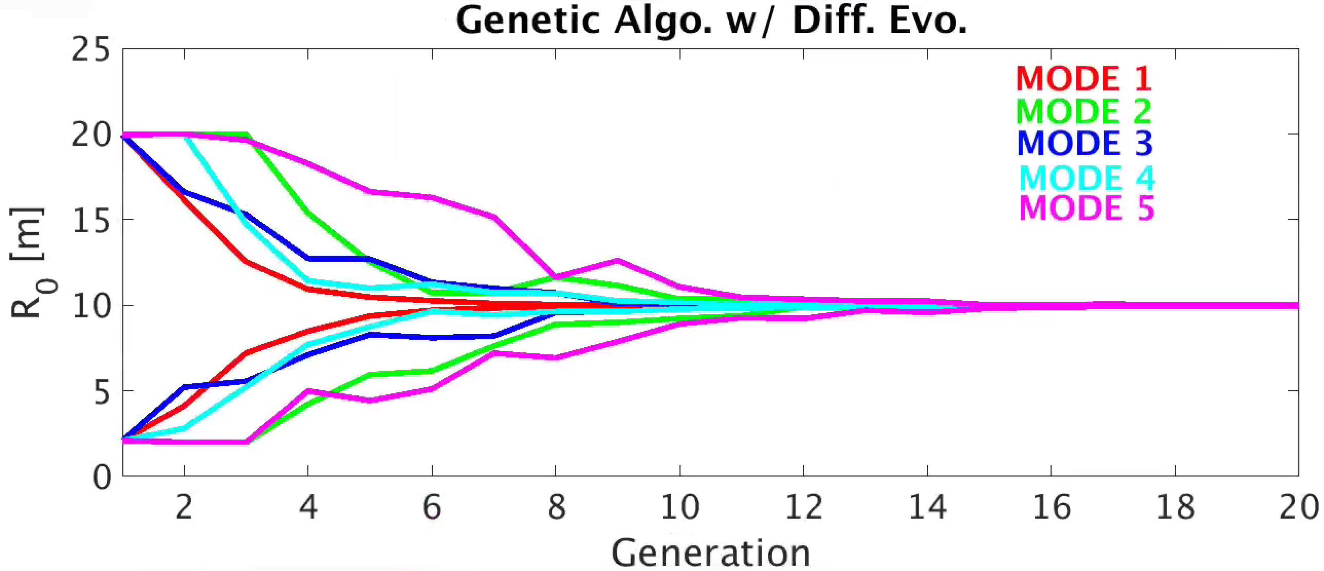
In this plot we show the upper and lower bounds of the population. It should be noted that since runs used the same random number seed, each population in generation 1 was the same, with a member with R0 approximately 10.03. Despite this we can clearly see the differences between choice of how the population converges on a minimum. Clearly MODE=1,3,4 appear to have the fastest convergence of the population. This can be attributed to their gene mixing algorithms including the most fit member of the population explicitly. Meanwhile MODE=2,5 do include this member explicitly. As a result their population take long to condense around the minimum. It should be noted that for this trivial problem the bounds for finding the global minima included the minima. In more realistic problems, the existence of many local minima may be missed by the choice of MODE=1,3,4. Choosing MODE=2,5 creates a more ‘search-like’ behavior.
The Particle Swarm Algorithm
In this section we evaluate the Particle Swarm Algorithm in STELLOPT. We will use the following OPTIMUM name list for STELLOPT:
&OPTIMUM
!------------------------------------------------------------------
! OPTIMIZER RUN CONTROL PARAMETERS
!------------------------------------------------------------------
  NFUNC_MAX = 25
  EQUIL_TYPE = 'VMEC2000'
  OPT_TYPE = 'PSO'
  FTOL = 1.0E-4
  XTOL = 1.0E-2
  FACTOR = 0.10
  EPSFCN = 0.5
  NPOPULATION = 16
  NOPTIMIZERS = 8
  LKEEP_MINS = T
!------------------------------------------------------------------
! OPTIMIZED QUANTITIES
!------------------------------------------------------------------
  LBOUND_OPT(0,0) = T
  RBC_MIN(0,0)=2.0
  RBC_MAX(0,0)=20.0
  RHO_EXP = 4
!------------------------------------------------------------------
! PLASMA PROPERTIES
!------------------------------------------------------------------
  TARGET_R0 = 10.0 SIGMA_R0 = 1.0
/
As for the Genetic Algorithm with Differential Evolution, bounding values on the variables are required. Our choice of parameters includes FACTOR, which defines the maximum step size of any particle in terms of the bounding space. In this case no particle can make a larger step than 10% the space. Here the bounds are 2 and 20 so no particle may make a step larger than 1.8 in RBC(0,0). The value of EPSFCN controls how large a step to take in the direction toward each particles local minimum. This value is relative to one for the step in the global minimum direction. If the value is set greater than one, each particle prefers to step towards its local minimum. For values of EPSFCN less than one the particles will step toward the global maximum. However care should be taken, the real formula used is: x(new) = x(old) + C*[x(global)-x(old)] + C*EPSFCN*[x(local)-x(old)] where x(old) is the current x-vector, x(global) is the global best x-vector, x(local) is the local best x-vector, and C is a random number from 0 to 1.